Basic Concepts of Spatial Relations #
The following contents are centrally stored in the geographic information system:
Spatial Distribution Location Information
Attribute information
Topological spatial relation information.
Thus, the description of spatial location, relationship and measurement plays an important role in GIS.
The spatial location relationship among geographical elements can be abstracted as the spatial geometric relationship among points, lines (or arcs) and polygons (regions), as shown in Fig. 3-12. Fig. 38 Partial Topological Spatial Relations among Geographical Elements # 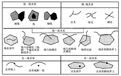
1) Point-point relationship
Consistency;
Separation;
One point is the geometric center of the other points;
One point is the geographic center of gravity of other points.
2) Point-line relationship
Point on a line: the properties of points can be calculated, such as inflection points, etc;
Endpoint of line: starting point and end point;
The intersection of lines;
Separation of point and line: The distance between point and line can be calculated.
3) Point-surface relationship
Points in the region can be counted and counted;
The point is the geometric center of the region;
The point is the geographical center of gravity of the region;
The point is on the boundary of the region;
The point is outside the region.
4) Line-line relation
Coincide;
Connection: First and last ring connection or sequential connection;
Intersect:
Tangent;
Parallel.
5) Line-surface relationship
Area containment lines: the density of lines in an area can be calculated;
Lines pass through the area:
Line surround with area: For the area boundary, the left and right area names can be searched;
Lines are separated from regions.
6) Surface-surface relationship
Contains: such as the island situation;
Coincide:
Intersection: Subareas can be divided and logical AND, OR, NOR and XOR can be calculated;
Adjacent: Calculate the nature and length of adjacent boundary;
Separation: Calculate distance, gravity, etc.
In recent years, there are many theories and applications of spatial relations at home and abroad. On the one hand, it provides the basic relationship for the effective establishment of GIS database, spatial query, spatial analysis and assistant decision-making. On the other hand, it applies spatial relation theory to GIS query language to form a standard SQL spatial query language, which can be used through API (Application Program Interface). Spatial features are stored, extracted, queried and updated.
Spatial relations include three basic types: topological relations, directional relations and metric relations.
Analysis of Topological Spatial Relations #
Topological attribute #
Topology comes from Greek, meaning “shape study”. Topology is a branch of geometry. It studies the topological attributes, which can remain unchanged under the topological transformation. In order to get some perceptual knowledge of the topology, it is assumed that the Euclidean plane is a high-quality, unbounded rubber, which can be stretched and shortened to any desired degree. Imagine a graph based on this eraser, allowing the paper to stretch but not tear or overlap, so that some attributes of the original graph will be retained and some attributes will be lost. For example, there is a polygon on the rubber surface and a point inside the polygon. Whether rubber is compressed or stretched, the point still exists inside the polygon, and the spatial position relationship between the point and the polygon does not change, while the area of the polygon will change. The former is the topological attribute of space, while the latter is not. Table 3-2 lists the topological and non-topological properties of objects contained in the Euclidean plane.
Table 3-2: Topological and Non-Topological Properties of Entity Objects on Euclidean Plane
Topological attribute | A point at the end of an arc An arc is a simple arc (the arc itself does not intersect) A point on the boundary of a region A point in the interior of a region A point is outside a region A point is inside a ring One face is a simple face (there is no island on it). Continuity of a surface ( given any two points on a surface, they can move from one point to another one along an arbitrary path completely inside the surface) |
Non-topological attributes | Distance between two points The direction in which one point points to another The length of arc Perimeter of an area Area of an region |
As can be seen from the table, the topological attributes describe the relationship between two objects, so they are also called Topological Relations. Figure 3-13 is a formal representation of topological spatial relations. Fig. 39 Points and neighborhoods in Topological Spaces # 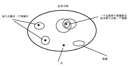
Mathematical Basis of Topological Description-Point Set Topology #
Topology is one of the branches of geometry. As a basic theoretical discipline of modern mathematics, it has penetrated into many branches of mathematics, physics, chemistry and biology, and has also been widely used in engineering technology. Because topology is the invariant property of graphics under the change of topology, it has become the theoretical basis of spatial relations in GIS. It provides a direct theoretical basis for describing spatial relations such as inclusion, coverage, separation and connection between points, lines and planes.
- Definition 1
\(X\) is a non empty set, \(\rho : X\times X \rightarrow R\) is a mapping, if for any \(x,y,z \in X\) , there is:
\(\rho(x,y)\ge 0\) , and \(\rho(x,y)=0\) , iff \(x=y\) ;
\(\rho(x,y)=\rho(y,x)\) ;
\(\rho(x,z) \le \rho(x,y) + \rho(y,z)\) (triangle inequality);
Then, ρ is called a metric on X , and the pair (X, ρ) is called a metric space.
- Definition 2:
Let A be a subset of a metric space X . If every point of A has a spherical neighborhood contained within A , then A is called an open set with respect to the metric ρ .
Definition 3: X is a non-empty sets, A is a subset family of X , if the following conditions are satisfied:
X and empty set Φ belong to A ;
(2)若*A1,A2*属于 A ,则 A1与A2 的交集属于 A ;
(3)*A*中任意两个元素的并仍为A中的元素;
It is called A is a topology of X . If A is a topology of collection X , the dual pair (X,A) is a topological space.
Definition 4: A is a subset of topological space X . If point x belongs to the every neighborhood U of X , and there are different points from x , such as U∩(A~{x})≠Φ , it is called the point of convergence or limit.. Agglomeration points of A either belongs to A or not belongs to A .
Definition 5: A is a subset of topological space X , the composed of all the gathering points of set A is called the derivative set of A and denoted as dX (A) or D (A)。
Definition 6: A is a subse of topological space X , if every gathering point of A belongs to A , the subset of A is d(A)*, the A is a closed set.
Definition 7: X is a topological space, the subset of X is the derived set of A and A , the union set A∪d(A) of d(A) is called the closure of A , it is noted a C(A) .
Definition 8: a subset of topological space X , if A belongs to neighborhood of X , the open set U of X belongs to U , U is a subset of A , so the point x is the interior point of A . A set of all interior points in A are called the interior of A, they are recorded as I(A) .
Definition 9: A is a subset of topological space X , if U which locates in any neighborhood of x exists the points of A and ~A , that is U∩A≠Φ and U∩(~A)≠Φ , the x is called the boundary point of A . A set of all boundary points (Collection A ) is called A Boundary, it is recorded as B(A) .
The theorem 1 : A is any subset of topological space X, then:
C(A)=~I(~A)=I(A)∪B(A)
I(A)=~C(~A)=C(A)~B(A)
B(A)=C(A)∩C(~A)=~(I(A)∪I(~A))=B(~A)
Topological Spatial Relation Description-9 Intersection Model #
There are two simple entities in the real world A and B, B (A) and B (B) represent the boundary of A and B, I (A) and I (B) represent the interior of A and B, E (A) and E (B) represent the surplus of A and B . Egenhofer [1993] structured a 9-Intersection Model,9-IM, comoposed of boundary, interior and remainder points , it is as follows:
B(A)∩B(B) | B(A)∩B(B) | B(A)∩E(B) |
I(A)∩B(B) | I(A)∩I(B) | I(A)∩E(B) |
E(A)∩B(B) | E(A)∩I(B) | E(A)∩E(B) |
For each element in the matrix, there are two values of “empty” and “non-empty”. A total of 9 elements can produce 2 9 =512 cases.
The 9-intersection model formally describes the topological relationship among discrete spatial objects. Based on the 9-intersection model, the consistency principle of spatial database can be defined and applied to database updating and maintenance. In addition, the 9-intersection model is also the basis for further study for spatial relations.
The 9-intersection model can express 512 possible spatial relationships, but in fact, some relationships do not exist. Table 2 gives the matrix forms of possible spatial relationships, including surface/surface (A/A), surface/line (A/L), surface/point (A/P), line/line (L/L), line/point (L/P), point/point (P/P). Whereas, “-” means that it is impossible to be this relationship, ‘Yb’ means the relationship that may exist on both single-valued and multi-valued vector graphs, and ‘Ym’ means the relationship that may exist on multi-valued vector graphs.
Table 3-3: Possible topological relationships between two elements represented by a 9-intersection model (in the table, nine values of the matrix are expanded to a binary value, ‘1’ indicates that the corresponding intersection is not empty, and ‘0’ indicates that the intersection is empty)
Relationship | 9-intersection model matrix | A/A | A/L | A/P | L/L | L/P | P/P |
|---|---|---|---|---|---|---|---|
r026 | 000011010 | Yb | |||||
r030 | 000011110 | Yb | Yb | ||||
r031 | 000011111 | Yb | Yb | Yb | |||
r063 | 000111111 | Yb | Yb | ||||
r092 | 001011100 | Yb | Yb | ||||
r093 | 001011101 | Yb | |||||
r095 | 001011111 | Yb | |||||
r127 | 001111111 | Yb | |||||
r159 | 010011111 | Yb | |||||
r179 | 010110011 | Ym | Ym | ||||
r191 | 010111111 | Yb | Yb | ||||
r220 | 011011100 | Ym | Yb | Ym | |||
r223 | 011011111 | Yb | |||||
r252 | 011111100 | Yb | |||||
r253 | 011111101 | Yb | |||||
r255 | 011111111 | Yb | Ym | ||||
r272 | 100010000 | Ym | |||||
r277 | 100010101 | Yb | |||||
r279 | 100010111 | Yb | |||||
r284 | 100011100 | Yb | Yb | ||||
r285 | 100011101 | Yb | Yb | ||||
r287 | 100011111 | Yb | Yb | Yb | |||
r311 | 100110111 | Yb | |||||
r316 | 100111100 | Yb | |||||
r317 | 100111101 | Yb | |||||
r319 | 100111111 | Yb | |||||
r349 | 101011101 | Yb | |||||
r373 | 101110101 | Yb | |||||
r400 | 110010000 | Ym | Ym | ||||
r412 | 110011100 | Yb | |||||
r415 | 110011111 | Yb | |||||
r435 | 110110011 | Ym | Ym | ||||
r439 | 110110111 | Yb | |||||
r444 | 110111100 | Yb | |||||
r445 | 110111101 | Yb | |||||
r447 | 110111111 | Yb | |||||
r476 | 111011100 | Ym | Yb | Ym | |||
r477 | 111011101 | Yb | |||||
r501 | 111110101 | Yb | |||||
r508 | 111111100 | Yb | |||||
r509 | 111111101 | Yb | |||||
r511 | 111111111 | Yb |
As can be seen from the table above, the number of possible topological relationships is far less than 512 (surface/surface: 6, surface/line: 19, surface/point: 3, line/line: 16, line/point: 3, point/point: 2). Figures 3-14 illustrate these possible relationships. In a sense, the topological relationship described by the 9-intersection model is only the category of the topological relationship. For each category, there are many possible situations, such as two intersecting lines, one intersection point and multiple intersections, which are consistent, but the topological relationship is different. Fig. 40 9-Intersection Model Topological Relation Diagram # 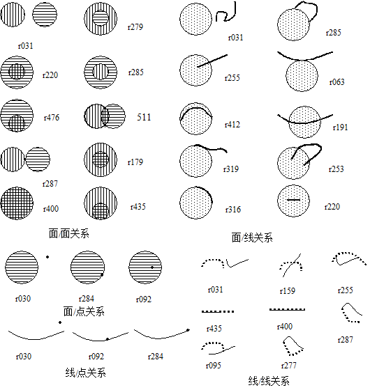
Extension of 9-intersection model
By introducing redundancy of point set, 9-intersection spatial relation model enhances the uniqueness of surface/line and line/line spatial relation. However, it only uses “empty” and “non-empty” to distinguish the boundary, interior and remainder of two targets, and there is little improvement in describing the spatial relations of face/face, point/point, point/line and point/surface. Therefore, this method still has some limitations.
In GIS, data can be divided into two types: geometric data and attribute data. Because of the measurability of geometric data, the objective world involved in Geographic Information System (GIS) is a metric space, and each metric space is a topological space. According to the degree of freedom of the target, the basic entity can be divided into three basic types: point, line and surface. Point target has fixed position and direction, which is defined as zero-dimensional target. Linear target has a tangible or invisible positioning line, which is defined as one-dimensional target. Surface target has a tangible or invisible contour line, which is defined as two-dimensional target.
The dimension expansion method is used to extend 9-IM, and the dimension of intersection among points, lines and surfaces, interior and remainder is used as the framework of spatial relationship description. For the boundary of a geometric entity, it is a set of lower one-dimensional geometric entities. For this reason, the boundary of a point is an empty set. The boundary of a line is two endpoints of a line, when the line is a closed curve, the boundary of a line is empty, and the boundary of a surface is composed of all the lines constituting the surface. If P is a set of points, the dimension function DIM of the set of points is defined as follows:
By using the dimension expansion method, the 9-intersection model can be extended to
DIM(B(A)∩B(B)) | DIM(B(A)∩I(B)) | DIM(B(A)∩E(B)) |
DIM(I(A)∩B(B)) | DIM(I(A)∩I(B)) | DIM(I(A)∩E(B)) |
DIM(E(A)∩B(B)) | DIM(E(A)∩I(B)) | DIM(E(A)∩E(B)) |
According to DE-9IM, for point set topological space X, when relational discrimination is needed, the 9-element values of the matrix can be analyzed and compared. Let C be the intersection point set of each unit, whose value P may be {T,F, 0, 1, 2} * . The specific meaning of each value is:
         P=T
         DIM(C)∈{0,1,2}
, the intersection C includes a point, line and surface;P=F DIM(C)=-1, means the intersection is NULL;P= DIM(C)∈{-1,0,1,2}, that is, the intersection of two objects with points, lines and surfaces, and some parts of the intersection is empty, which is generally not considered in relation discrimination;P=0 DIM(C)=0;P=1 DIM(C)=1;P=2 DIM(C)=2.
The elements in the extended 9-intersection model are selected by values
{T,F,\*,0,1,2}
, it can produce a situation of
       6^9
       =10077696
kinds of relationships, which are very complex. By summarizing and classifying a large number of spatial relationships, five basic spatial relationships are obtained: Disjoint, Touch, Cross, In and Overlap. These five relationships are defined as the minimum set of spatial relations, which are characterized by:
They can not be transformed into each other;
It can cover all spatial relation patterns;
It can be applied to geometric objects of the same dimension and different dimension;
Each relation corresponds to a unique DE-9IM matrix;
Any other DE-9IM relationship can be expressed by using these five basic relationships.
Topological Spatial Relation Recognition #
In GIS, spatial data has attributes, spatial characteristics and temporal characteristics. The basic data types include attribute data, geometric data and spatial relational data. As the basic data type, spatial relational data mainly refers to the relationships among points/points, points/lines, points/surfaces, lines/lines, lines/surfaces, and surfaces/surfaces.
Analysis of Directional Spatial Relations #
Direction Relation Description #
Directional relations, also referred to as orientation or extension relations, define the relative bearing between geographic objects. For instance, the statement “Hebei Province is located north of Henan Province” describes a directional relation. To define directional relations between spatial objects, we begin by establishing relations between point objects. Given a frame of reference consisting of mutually perpendicular X and Y coordinate axes, the definition of directional relations utilizes lines perpendicular to these coordinate axes as references. Let P :sub:`i` * be a point of target P (the primary object) and *Q :sub:`j` * be a point of target Q (the reference object), with functions *X(P :sub:`i` ) and Y(P :sub:`i` ) returning the X and Y coordinates of point * P i * , respectively. Then, between P and Q in two-dimensional space, there exist eight possible relations that provide a complete coverage of relationships. These relations are defined as follows:
Restricted_East(P :sub:`i` ,Q :sub:`j`)= X(P :sub:`i`)>X(Q :sub:`j`) And Y(P :sub:`i`)=Y(Q :sub:`j`)
Restricted_South(P :sub:`i` ,Q :sub:`j`)=X(P :sub:`i`)=X(Q :sub:`j`) And Y(P :sub:`i`)<Y(Q :sub:`j`)
Restricted_West(P :sub:`i` ,Q :sub:`j`)=X(P :sub:`i`)<X(Q :sub:`j`) And Y(P :sub:`i`)=Y(Q :sub:`j`)
Restricted_North(P :sub:`i` ,Q :sub:`j`)=X(P :sub:`i`)=X(Q :sub:`j`) And Y(P :sub:`i`)>Y(Q :sub:`j`)
North_West(P :sub:`i` ,Q :sub:`j`)=X(P :sub:`i`)<X(Q :sub:`j`) And Y(P :sub:`i`)>Y(Q :sub:`j`)
North_East(P :sub:`i` ,Q :sub:`j`)=X(P :sub:`i`)>X(Q :sub:`j`) And Y(P :sub:`i`)>Y(Q :sub:`j`)
South_West(P :sub:`i` ,Q :sub:`j`)=X(P :sub:`i`)<X(Q :sub:`j`) And Y(P :sub:`i`)<Y(Q :sub:`j`)
South_East(P :sub:`i` ,Q :sub:`j`)=X(P :sub:`i`)>X(Q :sub:`j`) And Y(P :sub:`i`)<Y(Q :sub:`j`)
The above eight relationships can be accurately judged by the projection of points. If there are any two points, the above eight relationships must have a satisfaction. Moreover, these relationships are transitive, and other relationships can be transformed to each other (such as North_East(PI,QJ)South_West(QI,PJ). By expanding the above eight relationships, four other directional relationships can be obtained, namely:
East(P :sub:`i` ,Q :sub:`j`)=North_East(P :sub:`i` ,Q :sub:`j`) Or Restricted_East(P :sub:`i` ,Q :sub:`j`) Or South_East(P :sub:`i` ,Q :sub:`j`)
South(P :sub:`i` ,Q :sub:`j`)=South_West(P :sub:`i` ,Q :sub:`j`) Or Restricted_South(P :sub:`i` ,Q :sub:`j`) Or South_East(P :sub:`i` ,Q :sub:`j`)
West(P :sub:`i` ,Q :sub:`j`)=North_West(P :sub:`i` ,Q :sub:`j`) Or Restricted_West(P :sub:`i` ,Q :sub:`j`) Or South_West(P :sub:`i` ,Q :sub:`j`)
North(P :sub:`i` ,Q :sub:`j`)=North_West(P :sub:`i` ,Q :sub:`j`) Or Restricted_North(P :sub:`i` ,Q :sub:`j`) Or North_East(P :sub:`i` ,Q :sub:`j`)
Based on the direction relationship between point targets, the direction relationship between other targets can be defined similarly.
Direction Relation Recognition #
MBR (Minimum Bounding Rectangle) refers to the tangent rectangle of a space target. The representation of MBR is very simple, just using two points (upper left corner and lower right corner). Because of its simplicity and practicability, MBR is widely used in spatial object data structure representation and spatial data query.
In order to determine whether there is a directional relationship between targets, we can first judge whether the MBR between targets has this relationship, and then use the point/point relationship to further judge the relationship and determine the specific relationship.
Analysis of Metric Spatial Relations #
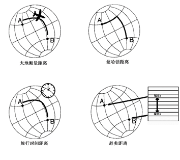
The basic spatial object metric relationships include the distance between points/points, points/lines, points/surfaces, lines/lines, lines/surfaces, and surfaces/surfaces. On the basis of the relationship between basic objectives, the metric relationship among point group, line group and surface group can be constructed. For example, on the basis of known point/line topological relationship and point/point metric relationship, the shortest path, optimal path and service range between points/points can be obtained. Known point, line and surface metric relationship can be used for distance measurement, proximity analysis, clustering analysis, buffer analysis, Tyson polygon analysis, etc. Quantitative measurement of spatial relationship between regional spatial indicators and regional geographic landscape is a unique capability of GIS. The regional spatial indicators include: Geometric indicators: location, length (distance), area, volume, shape, orientation and other indicators; Physical and geographical parameters: slope, slope direction, surface irradiance, topographic fluctuation, river network density, cutting degree, accessibility, etc; Indicators of human geography: such as concentration index, location quotient, difference index, geographic correlation coefficient, attraction range, transportation convenience, population density, etc. The distance between two points in geographic space can be measured along the actual surface of the earth or along the distance of the ellipsoid of the earth. Specifically, the distance can be expressed in the following forms (taking the distance between two cities on the earth as an example) (Fig. 3-15): Geodetic distance : The distance is the one that between two urban centers along the earth’s great circle. Manhattan Distance : Latitude difference plus longitude difference (the name “Manhattan Distance” is because the Manhattan, street patterns can be modeled as a set of two vertical lines). Travel time and distance : The shortest time from one city to another can be represented by a series of designated routes (assuming that each city has at least one airport). Dictionary Compilation Distance : The absolute difference between the locations of a series of cities in a fixed geographical list. Fig. 41 Distances of various forms on Earth # Measurement of Spatial Indicators #
Distance Measurement of Geospatial Space #