Spatial interaction and location-allocation model
Geographical position
For production units and service enterprises, there are always differences in spatial distribution between demand and supply, therefore, the selection and determination of Geographic Location of Institutional Facilities have a vital impact on their economic benefits and their own development.
The location evaluation and optimization of the facility is to optimize the spatial location distribution model by analyzing the interaction between the supply and demand of a facility or a facility network. Institutional facility location evaluation is an evaluation of the spatial location distribution pattern of existing service facilities, the optimization of institutional facility location is the search for its optimal location. Kristaqin’s central theory provides a basic framework for the theoretical research and application of empirical methods for the supply location optimization model, the market area size in this theory is determined by the scope of supply and service, and demand and supply, the relationship between the two is based on distance minimization and profit maximization. However, the central theory in practical applications, whether it is a theoretical method or its empirical methods, needs to be specifically analyzed according to specific problems. For example, contrary to the theory of the settlement world, the concentration and dispersion of the population in the region will have an impact on the size of the region; similarly, the choice of consumer behavior will also have an impact on the functional scope of a service center. Therefore, although the central theory provides a main framework for describing and interpreting the spatial interaction between the cargo service supply system and the demand behavior, it serves as a reference framework and needs to be expanded and adjusted for special situations. Figure 10-16 shows the conceptual framework for the application of central theory.
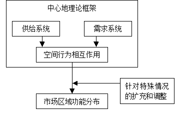
Figure 10-16: Conceptual framework for the application of central geography theory
The classical model of the central ground theory is a spatial analysis and simulation of a homogeneous functional area of the market that contains a single target and whose internal requirements are all directed at the target center, the modern model of central theory is to analyze and simulate the market functional areas of the real world that are uncertain and involve multi-objective consumption behavior and complex supply behavior.
Based on a more realistic study of market function behavior, many models have been developed for spatial analysis and simulation of real-world market functional areas, such as Reily’s Retail Gravitation, Batty’s Crack, Breakpoint Equation, Tobler’s Price Field and Interaction Wind, and numerous corrections. However, it is very difficult to use the gravity model and the crack point equation to analyze the multi-point center system. Due to the lack of visibility and continuity, the mapping of the analysis results is also difficult. The Tobler method is a semi-quantitative description of the characteristics of the central city market. Below, we will focus on a spatial linear optimization model for positioning-configuration problem solving.
Definition of spatial optimization pattern
The spatial optimization model is used to solve the location-allocation problem. Location-allocation problems arise when planning the location of important public facilities and their affiliated areas (public facilities, such as hospitals, kindergartens, playgrounds, nursing homes, schools, police stations, fire brigades, first aid stations, management facilities, etc., which belong to the infrastructure within the national budget).
A location-allocation problem can generally be expressed as follows:
There are a certain number of residential concentration points, which are called demand points (or consumption points, residential areas), and the demand distribution of a certain number of supply points (some public facilities) and/or supply points is sought to achieve a certain planning purpose.
If a demand point is set and a supply point is sought, the location or location problem is involved.
If a supply point is set up and allocation is sought, it involves allocation or allocation.
If both supply points and allocation are sought, the location-Allocation problem is involved.
Through the distribution between the demand point and the supply point, the subsidiary area of the supply point is also determined, as shown in Figure 10-17.
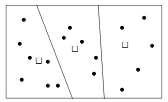
Figure 10-17: Location of public facilities and their affiliated areas
(The solid circle in the figure represents the demand point, and the box represents the supply point.
The boundary of the subsidiary area of the supply point is a simple straight line, but this is not the case in practice.
The optimization model basic structure consists of a series of boundary conditions and one (or several, but rare) objective functions. Under these boundary conditions, find the maximum or minimum of the objective function. Boundary conditions represent the conditions that must be met in planning objectives, and they represent a basic assessment of the function of the target planning area; optimizing the objective function (that is, finding the extremum of the objective function) represents a planning goal that is most likely to be achieved. Therefore, the planning conditions of the objective function reflected in the boundary conditions have the primary significance, the importance of the planning target corresponding to the optimization objective function is slightly worse, the significance of minimizing and minimizing the introduction of the objective function lies in obtaining a positioning, a clear answer to a configuration question (in the case where the objective function has several possible answers under certain boundary conditions).
Classification of spatial optimization patterns
According to the time range, problem space type, service mode of public facilities, road cost bearer and use type of public facilities, space optimization modes can be classified, as shown in Figure 11-18.
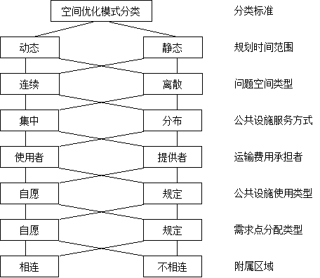
Figure 10-18: Spatial optimization pattern classification
Planning time frame
If the planning is to solve the location allocation problem in a certain period of time (point), the static optimization model is adopted. If the planning time range includes several time periods (points), the dynamic optimization model is adopted. Although the dynamic optimization model is easy to describe formally, it is difficult to achieve the optimization goal because of its large scale when it is used to solve practical planning problems. Many problems can be satisfactorily solved by static model.
Problem space type
If all the points in the study area are likely to be supply points, this is a continuous problem. But planning problems
In general, the number of supply points is limited, so the problem can be solved by discrete mode.
The two dimensions of planning time range and problem space type are very important because the corresponding pattern types are in shape.
The complexity of the structure, the possibility of problem solving and the operability of the model are quite different. The following will focus on “quiet”
State-discrete space optimization model, which can be further subdivided according to the facility types encountered in specific planning problems.
Service mode of public facilities
If public facilities are limited to providing services to the needy in a certain location, such as schools, kindergartens, nursing homes, hospitals, police stations, etc., the needy must go to these public facilities to receive services in person, the service mode of these public facilities is called “centralized”.
If the services provided by public facilities must be brought to the demanders by some means of transportation from the supply point, such as fire brigade, medical emergency center, police station, etc., the service mode of these public facilities is called “distributed”.
Transportation cost bearer
When the service mode of the public facilities is “centralized”, the demanders generally directly bear the cost of the journey to receive the services from these public facilities; when the service mode of the public facilities is “distributed”, the fees paid by the demander for receiving the service are generally independent of the distance traveled.
In the centralized location-distribution system, the accessibility of service supply points must be based on the viewpoint of social justice and equality of opportunity, while in the “distributed” location-distribution system, the consideration of work efficiency is more important.
Type of use of public facilities
Some public facilities, such as primary schools, hospitals, government management agencies, etc., are compulsory for those who need them based on relevant laws, such as nine-year compulsory education in primary schools, household registration management system, and unavoidable objective facts such as medical treatment. Because there are no competitors in this type of public facilities, their future demand and scale of facilities can be predicted, which is called prescriptive use type.
Other public facilities such as commercial buildings, restaurants, hotels, parks, stadiums and other social infrastructure are types of facilities that are voluntarily used. The contradiction between supply and demand of such facilities may become very prominent, therefore, their future needs and the scale of facilities are difficult to predict, and their demanders often change according to changes in transportation costs. When positioning such facilities, priority is given to selecting locations with a large increase in the number of residents.
Demand point allocation type
As with the use type of public facilities, the distribution type of demand points can also be voluntary or prescribed. In the “distributed” location allocation system, the distribution type of demand points belongs to the prescribed type, and the ancillary area composed of demand points belongs to public facilities is generally determined (even if the demand is voluntary); in the “centralized” location allocation system, the distribution type of demand points belongs to the voluntary type and belongs to the ancillary area composed of demand points of public facilities. Generally, it is uncertain.
It is more difficult to estimate the size of subsidiary areas and public facilities of each supply point under the condition of voluntary distribution of demand points. How to distribute users to supply points can be roughly estimated by the spatial interaction model with limited production and attraction.
Subsidiary area type
The prescribed distribution of demand points corresponds to the unrelated subsidiary areas, and the voluntary distribution of demand points corresponds to the connected subsidiary areas.
Mathematical expression of static-discrete space optimization model: linear programming
With regard to static-discrete positioning—configuration problems arise when planning the location of important public facilities and their associated areas. Static - discrete locations - configuration issues have to consider many potential supply points, and the determination of location and satellite areas will remain constant for long periods of time.
In the space optimization process, if the objective function and the boundary conditions are linear, the mathematical tool used is linear programming [1]_(Linear Programming). Linear programming refers to the problem of finding the maximum or minimum of a linear function under the constraints of a set of linear equations and inequalities.
The general form of linear programming is as follows:
Objectives:
Min c_1 x_1 + c_2 x_2 +… …+ c_n x_n
Constraints:
a_11 x_1 + c_12 x_2 +… …+
c_1n x_n ≤c_1
… …
a_m1 x_1 + c_m2 x_2 +… …+
c_mn x_n ≤c_1
x_1, x_2… … x_n ≥0
The following example belongs to the division of production and marketing, which can be solved by linear programming, there are three production areas A, B and C, with output of 50, 30 and 20 respectively, and demand of sales areas I, II and III is 40, 40 and 20 respectively. Firstly, through the shortest path analysis, the freight as described in Table 10-6 is obtained.
Table 10-6: Freight table for resource allocation (∞ indicates no connection)
I |
II |
III |
|
A |
2 |
3 |
5 |
B |
Infinity |
1.5 |
8 |
C |
2 |
4 |
Infinity |
The question is: how to determine the supply relationship, so that the total freight rate is the least. Assume that x:sub:`11`represents the traffic from A to I, x:sub:`12`represents the traffic from A to II, and so on. Then the problem can be described as:
Object:
Min 2x_11 +3x_12 +5x_13 +1.5x_22 +8x_23 +2x_31 +4x_32
Constraint:
x_11 + x_12 +x_13 =50
x_22 +x_23 =30
x_31 +x_32 =20
x_11 +x_31 =40
x_12 +x_22 +x_32 =40
x_13 +x_23 =20
x_11,`x_12,`x_13,`x_22,`x_23,`x_31,`x_≥0`
At present, there are many mature solutions to linear programming, such as solution method, simplex method and so on. The answer to the above-mentioned supply and marketing zoning is shown in Table 10-7, and the total freight is 255.
Table 10-7: Traffic volume of resource allocation
I |
II |
III |
|
A |
20 |
10 |
20 |
B |
0 |
30 |
0 |
C |
20 |
0 |
0 |
Genetic Algorithm:
Genetic algorithm is a recently proposed method for solving optimization problems, which optimizes the values of variables in a set to obtain a target that can quantitatively describe the pros and cons. The idea of quantifying the appropriateness of the target comes from Darwin’s theory of evolution, during the evolution process, the content and form of the genes of different generations of biological chromosomes are changing, making the organism more suitable for the living environment. In genetic algorithms, variables are changed by a combination of different ways and by modifying values, which is similar to the pairing and variation of organisms. By comparing the appropriate indicators, the results of the calculations after changing the variables are tested, the “favorable” combination is retained, and further modifications are made. An ideal result is that the retained changes are superior to other combinations and changes, and an iterative process can result in an optimized result. The success or failure of genetic algorithms depends on how the various forms of chromosomes are simulated and evolved to increase its chances of survival in the optimal solution.The surviving chromosomes generally correspond to a local extremum, which can lead to a global optimal solution.
In a genetic algorithm, the contents to be determined include:
Gene manipulation, such as pairing and mutation;
Strategic parameters: such as the probability of pairing and mutation;
Expression pattern: such as gene coding, etc.
In GIS, genetic algorithms can be applied to spatial interaction modeling, which can be applied to public facilities such as stores, hospitals, etc.