Raster data structure #
Definition #
Grid structure is the simplest and most direct spatial data structure. It refers to dividing the earth’s surface into uniform and closely adjacent grid arrays. Each grid is defined as a pixel or a pixel by rows and columns, and contains a code to represent the attribute type or magnitude of the pixel, or only a pointer to its attribute record. Therefore, the raster structure is a data organization that represents the distribution of spatial objects or phenomena by regular arrays, and each data in the organization represents the non-geometric attributes of objects or phenomena. As shown in Figure 7-4, in a grid structure, points are represented by a grid cell. A group of adjacent grid cells along the line of linear objects are represented by a maximum of two adjacent cells on the line. A surface or region is represented by a set of adjacent grid cells with regional attributes, and each grid cell can have more than two adjacent cells belonging to the same region. Remote sensing image is a typical raster structure, and the number of each pixel represents the gray level of the image.
(a)点 (b)线 (c)面 Fig. 90 The grid of points, lines and regions # 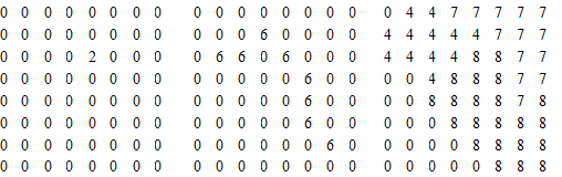
Characteristic #
The remarkable characteristics of raster structure are obvious attributes, implicit location, that is, data directly records the attributes of the pointer or attributes themselves, and the location is converted to corresponding coordinates according to row and column numbers, that is to say, location is based on the location of data in the data set. As shown in Figure 7-4-(a), data 2 represents a point of attribute or encoding 2 whose position is crossed by the third row and the fourth column where it is located. Because the grid structure is arranged according to certain rules, the position of the entities can be easily hidden in the storage structure of the grid file. When we talk about the encoding of the grid structure later, we can see that the row position of each storage unit can be easily obtained according to its record position in the file, and the row and column coordinates can be easily converted to coordinates in other coordinate systems. In a grid file, each code itself clearly represents the encoding of attributes or attributes of entities. If encoding of attributes, the encoding can be used as a pointer to the entity property table. As shown in Figure 7-4-(a), it represents a point entity with code 2, Figure 7-4-(b) represents a line entity with code 6, and Figure 7-4-(c) represents three plane entities or region entities with codes 4, 7 and 8, respectively. Because the raster row array is easy to store, operate and display for computer, this structure is easy to realize, the algorithm is simple, and easy to expand, modify, and also intuitive. Especially, it is easy to combine with remote sensing images, which brings great convenience to geospatial data processing.
The surface represented by the grid structure is discontinuous and is quantified and approximately discrete data. In the grid structure, the surface is divided into adjacent rectangular squares (triangles or rhomboids, hexagons, etc.) arranged regularly, and each block corresponds to a grid unit. The scale of raster data is the ratio of the raster size to the corresponding unit size of the surface. In many raster data processing, it is often assumed that the quantized surface represented by the raster is continuous, so that some continuous functions can be used. Because the grid structure quantifies the surface, when calculating the spatial indexes such as area, length, distance, shape and so on, if the grid size is large, it will cause greater errors. Because there may be more than one kind of ground object in the surface area of a grid, it is often a code in the corresponding grid structure. Similar to the mixed pixel problem of remote sensing imagery, such as Landsat MSS satellite imagery, each pixel in Landsat MSS satellite imagery represents a 79m × 79m rectangular area on the Earth’s surface, the spectral data recorded on the image is the sum effect of spectral radiation of all types of objects in the surface area corresponding to each pixel. Therefore, the errors may include not only morphological deformities, but also deviations in attributes。
How to determine the grid cell code #
When deciding the raster code, keep the authenticity of the surface as far as possible and ensure the maximum information capacity. A rectangular surface area shown in Figure 7-5, it contains three types of objects, A, B and C, O-point is the center point. When approximating the rectangular area as a grid element in the grid structure, the code of the grid element can be determined in one of the following ways as needed. Fig. 91 Determination of grid cell code # In the rectangular area shown in Fig. 7-5, the central point O falls within the area of the object coded C. According to the rules of the central point method, the corresponding grid unit code of the rectangular area is C. The central point method is often used for geographic elements with continuous distribution characteristics, such as rainfall distribution and population density map. In the example shown in Fig. 7-5, it is obvious that category B features occupy the largest area, so the corresponding grid code is set as B. The area dominance method is often used in the case of fine classification and small patches of land features. According to the importance of different objects in the grid, the most important type of objects is selected to determine the corresponding grid unit code. Assuming that the most important type of objects in class A in Figure 7-5, class A is more important than class B and C, the code of the grid unit should be A. Importance method is often used for geographic elements with special significance and small area, especially point and line geographic elements, such as towns, transportation hubs, transportation lines, River systems, etc. The code in the grid should express these important features as far as possible. The code of the grid unit is determined according to the percentage of the area occupied by the geographical elements in the rectangular area. For example, the two types of B and A with the largest area can be recorded, and the number can also be added to the code according to the percentage of the area occupied by category B and A.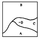
Center point method #
Area dominance method #
Importance method #
Percentage method #
Coding method #
Direct raster coding #
This is the simplest, intuitive and very important encoding method of grid structure. Usually, the encoding image file is called grid file or grid file. The logical prototype of grid structure is directly encoding grid file regardless of the compression encoding method used. Direct encoding is to treat raster data as a data matrix and record the code row by row (or column by column). Each row can be recorded from left to right, or even rows can be recorded from left to right, even rows can also be recorded from right to left, and other special order can be used for specific purposes (Figure 7-6). Fig. 92 Some of the commonly used grid ordering # 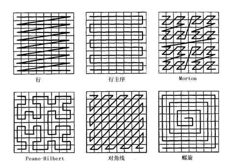
Compression coding method #
At present, there are a series of encoding methods for raster data compression, such as key code, run length encoding, block code and quadtree encoding. Its purpose is to record as much information as possible with as little data as possible, and its type can be divided into information lossless coding and information lossy coding. Information lossless coding means that there is no information loss in the coding process, and the original information can be completely restored by decoding operation. Information lossy coding means that data can be compressed to the maximum extent in order to improve the coding efficiency . In the process of compression, a part of the relatively less important information is lost, which is difficult to recover when decoding. Information lossless coding is often used in geographic information systems, and lossy coding is sometimes used in the compression coding of original remote sensing images.
1) Chain Codes
Chain Codes is also called [Freeman] chain code or boundary chain code, the chain code can compress raster data effectively, and it is very convenient for estimating area, length, concave and convex of turning direction, so it is more suitable for storing graphic data. The disadvantage is that it is difficult to modify and edit the boundaries, such as merging and inserting them. Local modification will change the overall structure, which is inefficient. Moreover, because chain code stores the boundaries of each area as a unit, the boundaries of adjacent areas will be stored repeatedly, resulting in redundancy.
2) Run-Length Codes
Run-Length Codes is an important encoding method for raster data compression. Its basic idea is that for a raster image, there are often several points adjacent to the row (or column) direction that have the same attribute code, so some method can be used to compress those duplicate records. There are two ways of coding: one is to record the code of each row (or column) and the number of repetitions of the same code in turn when the code of each row (or column) changes, so as to realize data compression. For example, for the raster data shown in Figure 7-4 (c), the following run length encoding can be performed along the direction of the line:
(0, 1), (4, 2), (7, 5), (4, 5), (7, 3), (4, 4), (8, 2), (0, 2), (4, 1), (8, 3), (7, 2), (0, 2), (8, 4), (7, 1), (8, 1), (0, 3), (8, 5), (0, 4), (8, 4), (0, 5), (8, 3).
Only 44 integers can be used to express the data, while 64 integers are needed to express the data in the direct coding mentioned above. It can be seen that run-length coding compressed data is very effective and simple. In fact, the compression ratio is inversely proportional to the complexity of the graph. In the part with more changes, the number of runs is more, and the part with less changes is less. The the graph is simpler, the compression efficiency is higher . Another run-length encoding scheme is to record the position and corresponding code of each row (or column) code change one by one. For raster data shown in Figure 7-4 (c), another run-length encoding scheme is as follows (along the column direction):
(1, 0), (2, 4), (4, 0), (1, 4), (4, 0), (1, 4), (5, 8), (6, 0), (1, 7), (2, 4), (4, 8), (7, 0), (1, 7), (2, 4), (3, 8), (8, 0), (1, 7), (3, 8), (1, 7), (6, 8), (1, 7), (5, 8).
When the Run-Length Codes in raster is compressing, the amount of data does not increase significantly, compression efficiency is high and easy to retrieve, overlay and merge, the operation is simple, the suitable for machine storage capacity is small, data needs a lot of compression, but also to avoid complex coding and decoding operations increase processing and operation time.
3)Block Codes
Block Codes is a case where run-length encoding is extended to two dimensions. A square area is used as the recording unit. Each recording unit includes several adjacent grids. The data structure consists of the initial position (row, column number) and radius, together with the code of the recording unit. The block code coding of the image shown in Figure 7-4 (c) is as follows:
(1,1,1,0), (1,2,2,4), (1,4,1,7), (1,5,1,7),
(1,6,2,7), (1,8,1,7), (2,1,1,4), (2,4,1,4),
(2,5,1,4), (2,8,1,7), (3,1,1,4), (3,2,1,4),
(3,3,1,4), (3,4,1,4), (3,5,2,8), (3,7,2,7),
(4,1,2,0), (4,3,1,4), (4,4,1,8), (5,3,1,8),
(5,4,2,8), (5,6,1,8), (5,7,1,7), (5,8,1,8),
(6,1,3,0), (6,6,3,8), (7,4,1,0), (7,5,1,8),
(8,4,1,0), (8,5,1,0).
In this example, 120 integers are used for block codes, which is more than direct coding. This is because in order to describe conveniently, the grid division is very rough. In practical application, fine grid division and more data redundancy can show the effect of compression coding, and some technical processing can be done, such as line number can be marked between lines without recording, line number and radius need not be double bytes. Integer records can further reduce data redundancy.
Block codes have variable resolution, that is, when the code changes little, the block size is large, that is to say, the internal resolution of the area patches is low. On the contrary, the high resolution records the boundary areas of the area with small blocks, so as to achieve the purpose of compression. So block code is similar to run-length coding, which reduces the efficiency with the increase of the complexity of graphics, that is to say, the pattern is larger, the compression ratio is higher. The fragmented pattern is more, the compression ratio is lower. Block codes have obvious advantages in merging, inserting, checking extensibility and calculating area. However, in some operations, run-length coding and block code decoding must be converted into basic raster structure.
4) Quadtree
Quadtree, also known as quaternary tree or quarter tree, is one of the most effective encoding methods for raster data compression. Most graphics operations and operations can be implemented directly in quadtree structure. So quadtree encoding not only reduces the amount of data, but also greatly improves the efficiency of graphics operations. Quadtree decomposes the whole image area into a series of square areas which are contained by a single type of region. The smallest square area is a raster pixel. The principle of segmentation is to divide the image area into four quadrants of the same size, and each quadrant can be divided into four quadrants of the next level according to certain rules. As long as the upper quadrant is divided into only one kind of object or a few kinds of objects that meet the established requirements, it will not continue to divide, otherwise it will be divided into a single grid pixel, no matter which level it is. Quadtree records this partition through tree structure, and implements query, modification, measurement and other operations through this quadtree structure. Figure 7-7 (b) is a quadtree decomposition of Figure 7-4 (c). The scales of each sub-quadrant are not exactly the same, but they are all the same as the code grid units, the quadtree is shown in Figure 7-7-(c). Fig. 93 Block Code Segmentation; Quadtree Segmentation # Fig. 94 B quadtree coding # Quadtree coding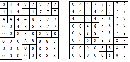
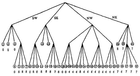
The top node is called the root node, which corresponds to the whole graph. There are four layers of nodes, each of which corresponds to a quadrant. For example, two layers of four nodes correspond to the four quadrants of the whole figure respectively. The order of arrangement is SW, SE, NW and NE. The nodes that can not be separated are called termination nodes (also known as leaf nodes), which may fall on different layers. The sub-quadrants represented by this node have a single generation. Code, the square area represented by all termination nodes covers the whole figure. From top to bottom, the number of leaf nodes from left to right is shown in Figure 7-7 (c). There are 40 leaf nodes, that is, the original map is divided into 40 square sub-areas of different sizes. The bottom row of numbers in Figure 7-7 (c) represents the code of each sub-area.
From the quadtree decomposition of the above figure, it can be seen that the size of quadrants in quadtree is different. Quadrants located at higher level are larger, and the number of decomposition times is less when the depth is small, while quadrants at lower level are smaller, and the number of decomposition times is more when the depth is large. This reflects that the distribution of single objects in some locations on the map is wider, while those at other locations are more complex and changeable. It is precisely because quadtree coding can automatically adjust the quadrant size according to the graph changes, so it has a very high compression efficiency.
When quadtree coding is used, in order to ensure that quadtree decomposition can continue, the image must be raster array 2 n ×2 n , ‘n’ is the limit segmentation number, ‘n+1’ is the maximum height or layer of quadtree. Figure 7-4(c) is the raster 2 3 ×2 3 , so it is divided into 3 times, maximum is 4 times. For non-standard size images, the first step is to expand the image 2 n ×2 n 。
In order to make the computer not only store quadtree corresponding to image with minimum redundancy, but also complete various graphics and image operations conveniently, experts have proposed various coding methods. The following is an introduction to the coding method adopted in the Geographic Information System of the University of Maryland in the United States. This method records the address and value of the termination node (or leaf node). The value is the code of the subregion. Address consists of two parts, 32 bits (binary). Four bits on the right record the depth of the leaf node, at the level of the quadtree, the size of the subarea can be inferred by the depth. Address is represented by the path from the root node to the leaf node, 0, 1, 2, 3 represent SW, SE, NW, NE respectively, and 2n bytes from the fifth bit on the right record these directions. As shown in Figure 7-7-(c), the sixth node depth is 3, the first layer is in the SW quadrant, which is 0. The second layer is in the NE quadrant, which is 3. The third layer is in the NW quadrant, which is 2:
0000… 000 (22); 001110 (6); 0011 (4)
Each quadrant position is represented by two binary digits, a total is 6 bits, and a decimal integer is 227. In this way, the address of each leaf is recorded, and then the corresponding code value is recorded. This image can be recorded and various image operations can be carried out on the basis of this coding.
In fact, the address of leaf nodes can be obtained directly from the row coordinates of the lower left corner of the sub-region, interlaced by binary bits. For example, in the row coordinate system with the lower left corner of the image as the origin, the row and column coordinates in the lower left corner of the image are (3,2), which are expressed as binary 011 and 010, respectively, and the staggered position is 001110, which is the block 6.
In order to improve the efficiency of maps with only point objects or linear objects, a slightly different division termination conditions and recording methods are designed, which are called point quadtree and line quadtree. The point quadtree divides the sub-quadrants until each sub-quadrant contains no point or only one point. The leaf value records whether there are points and points in the sub-quadrant. The line quadtree divides the sub-quadrant until the sub-quadrant contains no line segment or only a single line segment. The node of the line divides into a single pixel, and the leaf value record is more complex.
Quadtree coding has variable resolution, regional property and flexible data compression. Many operations can be directly implemented on the encoding data, which greatly improves the operational efficiency and it is one of the excellent raster compression coding.
Generally speaking, data compression is at the cost of increasing computing time. Time and space are a pair of contradictions. In order to utilize space resources more effectively and reduce data redundancy, more computing time has to be spent on coding. A good compression coding method is to achieve the maximum data compression efficiency on the basis of minimizing computing time as much as possible, and the algorithm is adaptable and easy to implement. Chain codes have high compression efficiency and near vector structure, which are convenient for boundary operation, but they do not have the nature of region and are difficult to operate in region. Run-length coding can compress data to a large extent, and retain the original raster structure to the maximum extent. It is very easy to code and decode. Block codes and quadtree codes have the nature of region and variable resolution. Quadtree coding is a promising method because of its high compression efficiency, which can directly perform a large number of graphic and image operations. On this basis, octree coding for three-dimensional data has been developed.